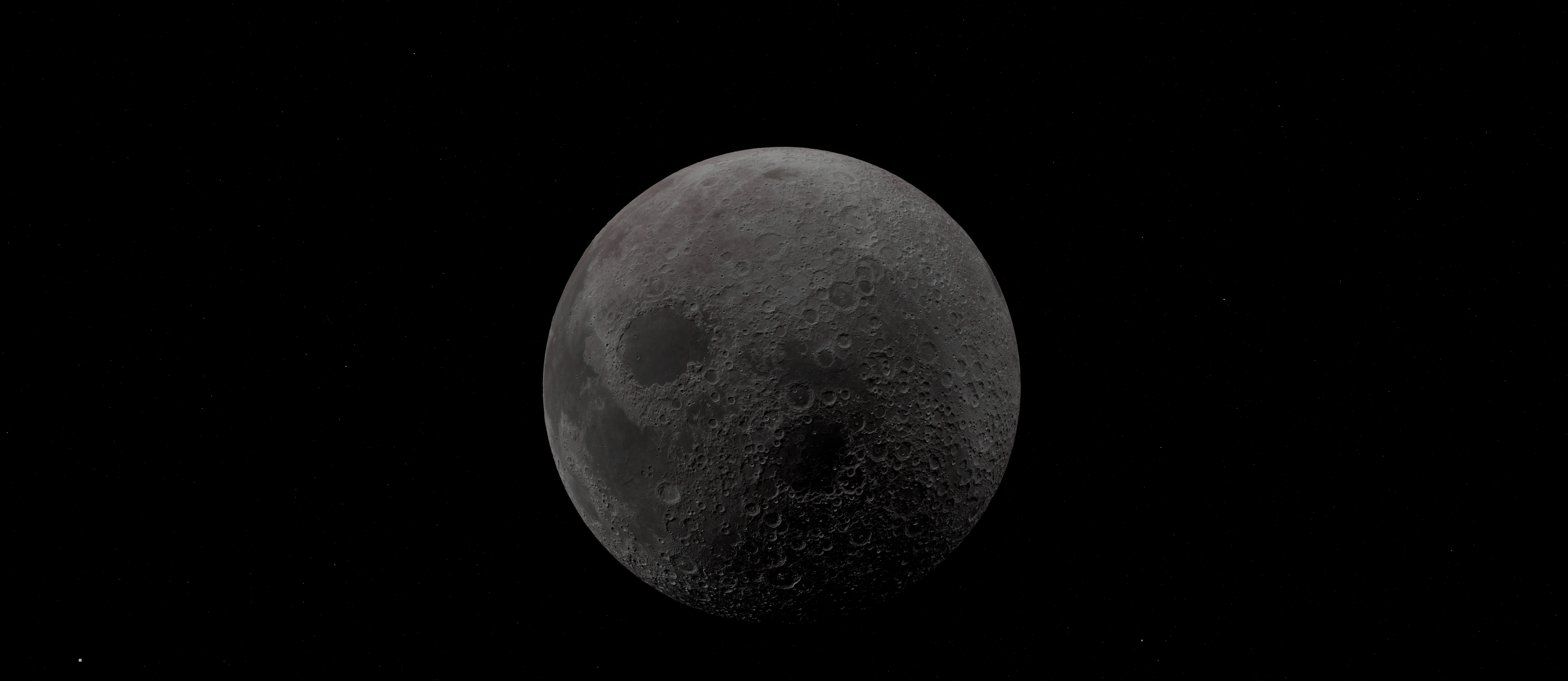
DATASET: CHANG'E-2 DEM
RESOLUTION: 20 M / PX
ENGINE: UNREAL ENGINE 5.8
MOON // GLOBAL VIEW
aria-label="Navigation controls and surface exploration video">
▶
aria-label="Mineral map features and overlays video">
▶
aria-label="Surface flyover of the CE2 and SLDEM2015 elevation difference map">
▶
▶
OVERVIEW
PROJECT ORIGIN
AND SCOPE
The core of this project relies on the Chang'E-2 (CE2) 20 m/px digital elevation model (DEM). The
mission was undertaken by the China National Space Administration (CNSA) and launched on October 1,
2010, with the goal of capturing high-resolution images of the Moon's surface for potential future
landing sites.
I want to start off by stating that I'm a procedural 3D artist jumping into the scientific
visualization field, not a planetary researcher or a software engineer. My goal was to build a 1:1
digital twin of the Moon at the highest resolution that I thought was possible.
[Note]: I now know it can get much higher and better, using a similar method as Casey Handmer did to
build the 7.2 m/px map of Mars. He did not share the technique or algorithm, but I'm confident I
could figure it out if I ever do another project like this.
This meant diving into a lot of math and data processing that I had zero background in. I had to
learn a lot of it on the fly, which is actually my preferred way of learning anyway.
The one thing I made an executive decision not to learn was how to actually code. I started the
project by dipping my toes into coding bootcamps, YouTube tutorials, etc., but very quickly realized
it was a massive waste of time. AI was advancing at such a rapid pace that, if I'm being honest, I
would never catch up to it, let alone get anywhere close. Trying to hand-write code when it could be
done much faster and, in many cases, better using LLMs just didn't seem like a smart way to approach
the project.
Instead, I decided to take more of a "learn to read the code" approach. I still needed to understand
the broad concepts, algorithms, and theories behind what I was doing, because I can't just say "hey
computer, figure this out" and expect it to magically work. It's more like: "Use this algorithm on
this dataset. I need this specific result, and for that to work, I need XYZ in this format with this
particular attribute. Make that happen."
The AI handles the lower-tier implementation and code writing while I handle the higher-tier
thinking, planning, and assembly. I don't need to know how to manually write every line of code if I
understand what the code needs to accomplish, why it needs to work that way, and how to recognize
when it isn't doing what I intended.
[Note]: But a massive piece of advice—never blindly trust AI code. Always verify it two or three
times over to make sure it's actually doing what you need. This may seem obvious, but it is
imperative. LLMs can easily reverse a sign, produce an approximate or fabricated value, or introduce
other subtle errors that are easy to miss.
Here is a breakdown of how this project actually came together, from raw data to a real-time Unreal
Engine environment.
PHASE 01
DATA SELECTION
STANDARDIZATION
Initially, I intended to just grab the elevation data from the NASA Trek portal, which hosts the
dataset pre-converted to an Equirectangular projection. But when I brought it in, the dataset had
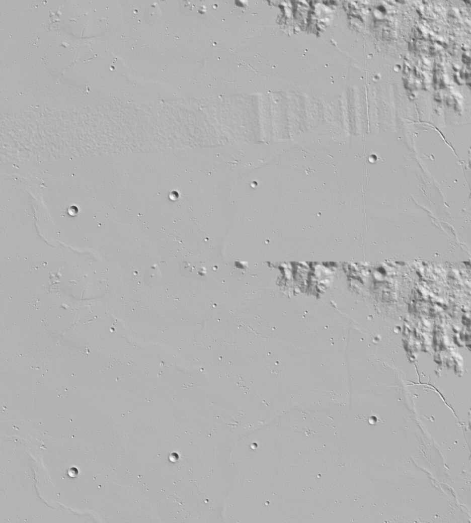
two massive structural flaws. First, their reprojection pipeline introduced huge "NoData" pixel
bloat (Figure-01). This turned a perfectly fine 2–3 GB file into a 15–30 GB monster, and some tiles
artificially spanned the entire lunar equator. Second, the equatorial tiles displayed a very
specific 7-degree latitudinal compression (Figure-02)
It turns out the native CE2 metadata uses a Mercator_2SP projection with a Standard_Parallel_1 of
7.0, and the NASA pipeline just completely omitted that setting during reprojection. I couldn't
continue the project on broken foundations, so I pivoted to the raw data hosted by the National
Astronomical Observatories of China (NAOC).
The raw NAOC archive comprised 180 32-bit float GeoTIFFs scattered across different projections.
These too had flaws, the first being that the metadata inside the actual files was seemingly
incorrect. The good news was that they came with .prj and .tfw sidecar files that contained the
correct metadata, so I overrode the internal metadata with them. The second issue was that a lot of
the files had slightly different NoData pixel values ranging from -3.4028234e38 to -3.4028235e38.
Some even had their metadata say that the NoData value was -3.4028234e38, but in reality, it was 0.
[Note]: This caused a lot of confusion, and it took time to figure out that this was even happening
because leaving those zeros unpatched would generate solid geometry walls at the tile boundaries
when resampling.
I did a full metadata cleanup, unifying all the NoData pixel values. I now had the dataset cleaned
and ready to build into a digital twin inside Unreal Engine... or so I thought.
FIG 01 // NODATA PIXEL BLOAT
[Note]: Example of NASA Trek NoData pixel bloat, out of all the pixel only a very small portion is
real data (Red pixels = NoData)
FIG 02 // Conpression at the equator
[Note]: Equatorial tile compression resulting from the omitted 7-degree standard parallel during the
reprojection.
PHASE 02
DYNAMIC FREQUENCY
ISOLATION
While working on the project, I stumbled upon a research paper that talked about the dataset I was
working with, and it highlighted some anomalies and errors within it, along with some theoretical
fixes. Like always, I couldn't help myself but to try and implement them (a costly mistake).
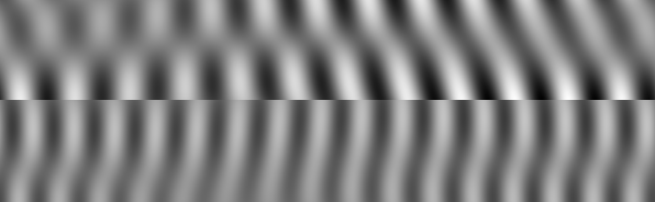
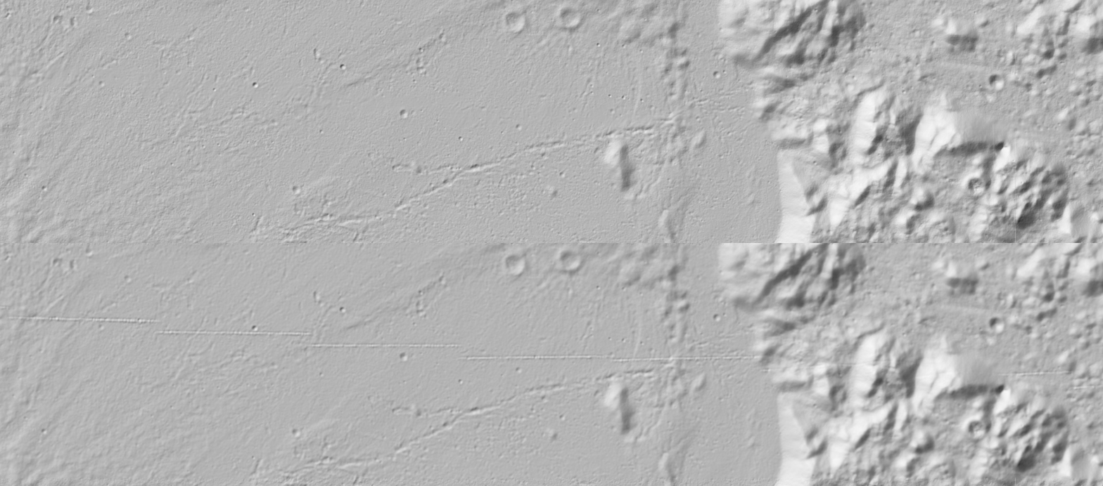
The CE2 data has these weird periodic orbital ripples baked into the terrain. Research by Xin et al. (2020) identified
these orbital ripples and approximated their wavelength at 21 km (Figure-03). I attempted to use
that 21 km value to fix the ripples but realized that it was not precise enough for widespread
correction. The ripples change in width and strength depending on the topology of the terrain, pole
compression, elevation, etc. After testing, I found out that the spatial frequency ranges from 8 km
all the way up to 45 km.
FIG 03 // Ripple Error
[Note]: This is a difference map of a single tile where you can clearly see the ripples in question.
To capture the ripples without destroying real terrain details, the frequency separation needed to be
dynamic. First, an SLDEM2015 baseline map (currently the gold standard, with a vertical accuracy of
~3 to 4 meters and horizontal geolocation errors adjusted to less than 10 meters, at a 60 m/px
resolution) is subtracted from the CE2 terrain to isolate the raw geometric noise. This allows the
isolation of the large-scale detail where the ripples live from the small difference in topology
that exists between two datasets with such large resolution deltas. A 2D Hanning window (bell curve
that fades to 0) smooths the edges, and 4x zero-padding sharpens the frequency resolution, both
applied before the discrete Fourier transform, so the true peak isn't masked:
The resulting power spectrum is then scanned for a peak somewhere between 8 km and 45 km for each
specific tile. Once found, the Full Width at Half Maximum (FWHM) is extracted to calculate the exact
center frequency \( f_c \) (the peak value) and bandwidth \( B \) (the width of the frequency):
To make sure we don't accidentally nuke the good high-frequency topography (like the actual craters),
this filter is restricted by a directional wedge mask. For the cross-track ripples, the cut is only
applied where the angular frequency \(\theta = \arctan(v/u)\) falls within 3° of the primary orbital
axes. The rest of the frequency space is left completely untouched.
Multiplying this constrained mask by the transformed terrain difference and running an inverse
transform isolates the exact ripple energy. Subtracting that exact energy profile from the raw CE2
data flattens the periodic artifacts, but the native craters stay crisp. The filter parameters were
kept intentionally conservative to leave a tiny fraction of the ripple intact rather than risk
blurring real elevation features. It basically pushes the artifact below the threshold of what you
can actually see in the final 3D build.
To actually quantify whether this dynamic notch filter worked (and prove I didn't just ruin the data
by doing some bs), a comparative spectral analysis was run on the CE2 DEM before and after
correction. The validation metric relies on the power spectral density \(P(u, v) = \vert F(u, v)
\vert^2\), defining the signal-to-noise ratio of the artifact as \(R =
\frac{P_{peak}}{\text{median}(P_{range})}\). Here, the denominator is just the median power of the
real terrain frequencies within that 8 km to 45 km search window.
Prior to filtering, these orbital artifacts dominated the spectrum. Pre-correction scans were hitting
distinct periodic peaks exceeding a 2.0x baseline detection threshold almost everywhere, frequently
averaging over 200x the local noise floor. After applying that conservative Butterworth wedge mask,
the full detection scan was re-run on the corrected terrain. The ripples were successfully removed,
dropping the ripple power below the 2.0x detection threshold for over 98% of the processed tiles.
(For the rest of the files that didn't get such good results, I just let them be. I could not find
why they were outliers, and I had already spent way too much unnecessary time on this part.)
Finally, by computing the Root Mean Square (RMS) of the subtracted ripple array:
I could verify that the geometry removed from the raw DEM strictly matched the isolated orbital
noise. This verifies that the removed component corresponded to the isolated orbital noise rather
than an arbitrary modification of the surrounding terrain.
[Note]: The reason I said doing this was a costly mistake was the fact that it took me 2 months to
figure it out and in the end it was pointless. Like I stated in the beginning, I'm not trying to be
a planetary scientist, and my job isn't to correct the data in that way, its to visualize the data.
At most I should tweak how the data looks visually, but I should not change the underlying data if
it does not affect how the project looks in the end.
The next section's fixes are more of what I should be doing. Although I do have to admit it was very
fun tinkering and losing my mind trying to figure it out, you can't be and do everything, I had to
stick to the real task at hand.
PHASE 03
Topological Restoration
Beyond the ripple, the dataset had some processing or scanning artifacts that were identified by Xin
et al. as gross errors. These errors needed a more surgical approach to fix (the fun part).
I approached this like a compositing trick in Photoshop, but using spatial-frequency separation in
3D. I masked the corrupted regions and separated both the CE2 data and the SLDEM2015 reference data
into low-frequency base shapes and high-frequency textural details using a Gaussian filter \(\sigma
= 3.0 px\). I threw away the corrupted CE2 base, vertically aligned the SLDEM2015 base to fit
perfectly, clamped the CE2 high-frequency details to a strict \(\pm 0.3 m\) threshold (to kill any
outlier spikes), and blended it all back together with a smooth 64-pixel Gaussian weight map. It
patches the terrain seamlessly without tearing the geometry.
After fixing all the known errors, it was finally time to mosaic the individual files together.
Because the original CE2 tiles were processed independently, the overlapping edges (skirts) drifted
slightly in elevation. If you just stitch them together normally, you get massive step artifacts at
every single boundary. To fix this without breaking the topology, I ran the dataset through the Ames
Stereo Pipeline (ASP).
[Note]: ASP is a really cool tool with an insane amount of utility. I only discovered it much later
in the project after trying a million and one different ways of fixing the seams created by the tile
skirts. It's built to only work on Linux systems at the moment, so if you are on Windows, you have
to use WSL to get it running.
I used its dem_mosaic tool, which applies a distance-weighted blending algorithm. Basically, it
calculates a continuous weighted average based on how close a pixel is to the center of its original
tile. It perfectly smooths out the elevation drift across the seams, giving you one buttery-smooth,
continuous surface.
PHASE 05
ADAPTIVE DECIMATION
AND ENGINE OPTIMIZATION
Loading a 20 m/px global elevation model natively into a real-time engine is just asking a regular PC
to commit seppuku or gain sentience to choke you out. That is about 59.9 billion vertices and 3.35
TB, not even accounting for UVs, normals, etc.
To give you an idea of how heavy this is: I tried loading just a single uncompressed full-resolution
tile (an RTIN error of 0) to compare it, and it was nearly 16 GB. Even after converting to GLTF, it
was 6 GB (which doesn't really matter anyway because Unreal Engine uncompresses the files on
import). Houdini and Unreal Engine crashed instantly, running completely out of memory, and my rig
has 64 GB of RAM.
To make this run, I used a Right-Triangulated Irregular Network (RTIN) algorithm to decimate the
mesh. Setting the error tolerance to 2.0 meters collapsed the flat areas but perfectly preserved the
crater rims and semi-micro terrain Topological. It shed 96.5% of the geometry, dropping the total
size to a much more manageable 118.7 GB.
[Note]: The reason for such a massive reduction is that 20 m/px doesn't mean every pixel contains
meaningful geometric detail. Some neighboring pixels can differ by less than 0.01 m in elevation, so
removing those tiny differences is effectively imperceptible while saving a massive number of
vertices.
I baked tangent-space normal maps from the raw data to keep the micro-details looking sharp. The
combination of those two allowed me to save an ungodly amount of space and **computational
overhead** (or GPU horsepower, if you prefer), while keeping the terrain looking nearly identical to
the full-resolution mesh.
Inside Unreal Engine 5, the native HLOD system was giving me terrible popping and seams. So, I built
a custom C++ subsystem (`UWorldPartitionRuntimePlanetaryHash`) that streams LODs based strictly on
vertical distance and the camera's angle to the horizon, bypassing the standard bounding-box
streaming entirely. The native Unreal Engine tools work amazingly well on regular "flat" terrains,
but they start to break down and get overly complicated when working with spherical planetary
bodies. Luckily, they provide the tools to build your way around it with custom C++ (I'm a big fan
of Unreal Engine).
PHASE 06
TEXTURE SYNTHESIS
AND GEOLOGY
The project relies on a few different types of visuals. The first is the base albedo (color) map. For
this, I used the NASA CGI Moon Kit color map . It is
the closest thing you will find to a perfect, full-moon color map. It doesn't have baked-in shadows,
processing artifacts that ruin the colors, or massive missing chunks like other datasets I tried. It
does have one downside: it has an effective resolution of 398 m/px, which was significantly coarser
than the rest of my project.
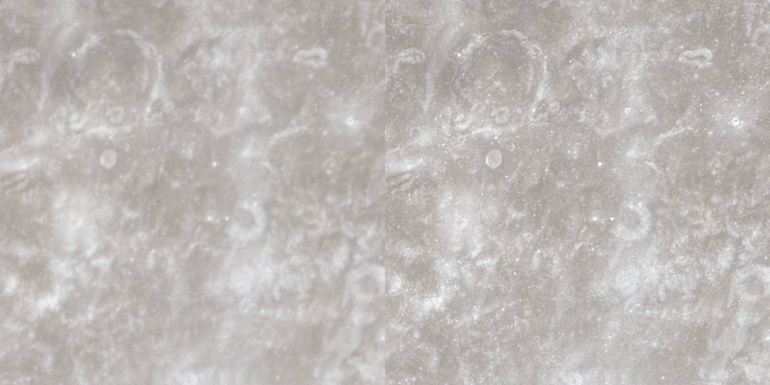
To fix this, I found the WAC_EMP_643NM_E000N0000_304P map from the
Lunar Reconnaissance Orbiter Camera (LROC). Because this is a near-global reflectance map, I decided
to use it to modulate the pixel brightness of the low-res CGI Moon Kit. This essentially upgraded
the map's resolution to 98 m/px, a beautiful 4x increase in detail without introducing any fake,
AI-generated upscaling data (Figure-06A). To my surprise, this enhancement also nicely cleaned up
some clear visual artifacts that were present in the original CGI map (Figure-06B)
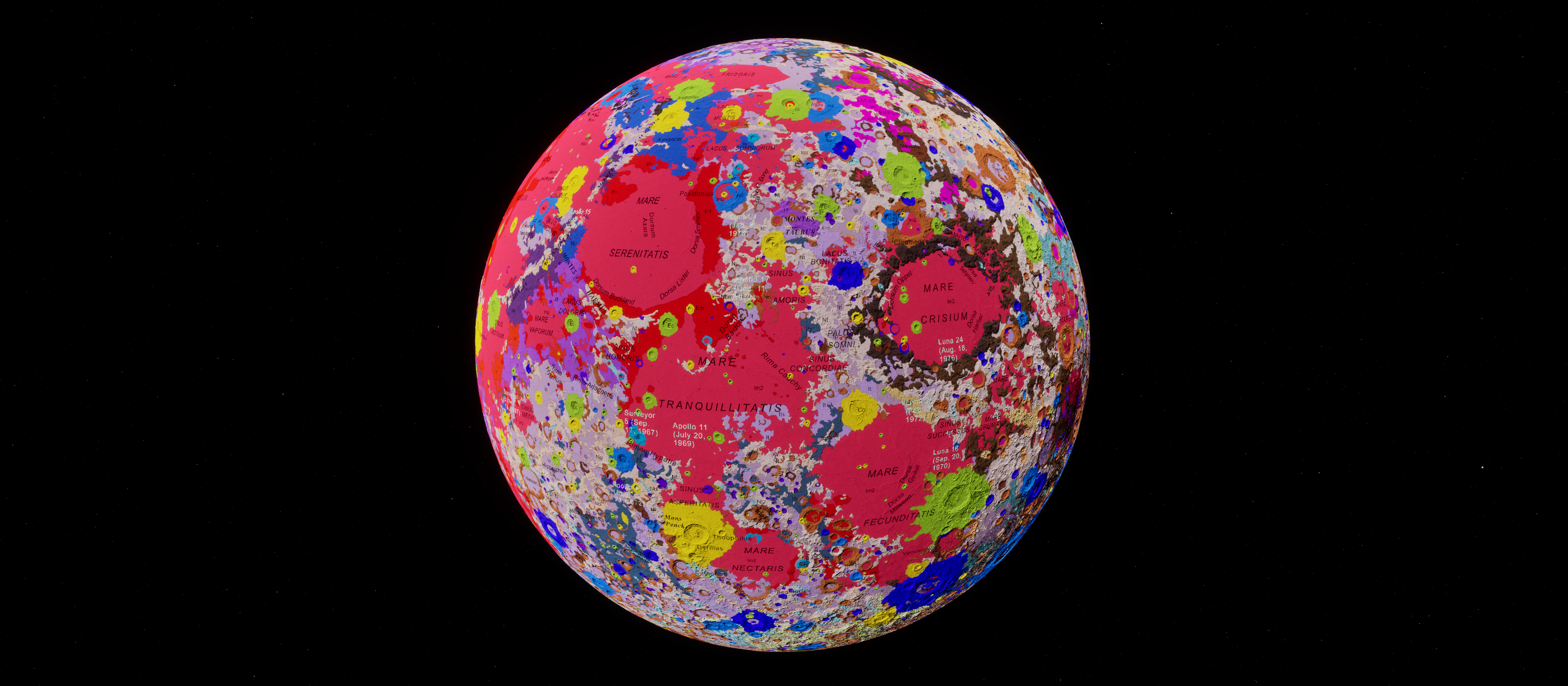

The next visual I integrated was the 1:5,000,000 USGS Unified Geologic Map (Figure 07). Rather than
just slapping the image onto the globe, I separated all of its components into multiple textures.
This allowed me to set up the Unreal Engine material so I could toggle specific sections on or off
on the fly. You can flip a switch to see linear features, crater names, landing sites, etc. Every
distinguishable feature within those maps has a specific value assigned to it, meaning they are
individually toggleable. For example, I can filter the map to hide all craters with a diameter of
less than 30 km
FIG 07 // USGS Unified Geologic Map
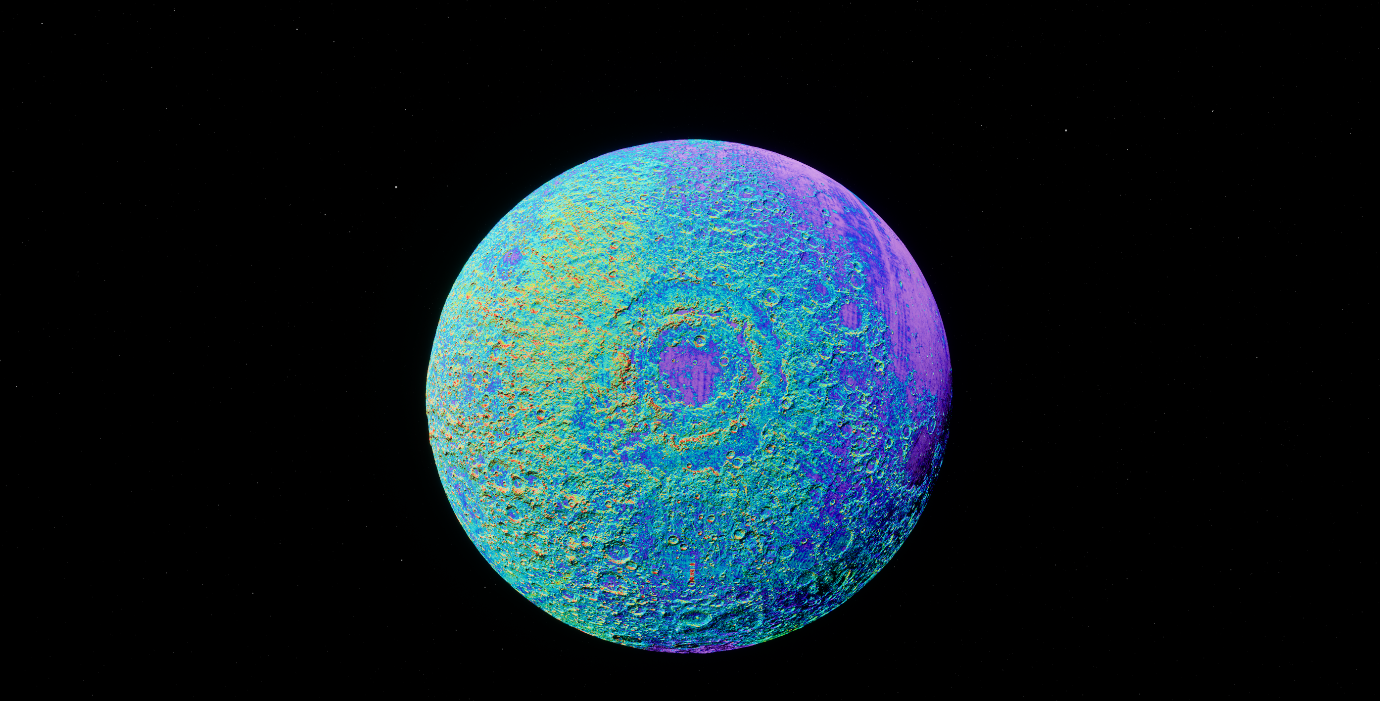
For the last map, I wanted to visually expose the actual differences between the CE2 terrain and the
SLDEM2015 reference map. I mapped the elevation differences into an 8-bit layer that applies a stark
color gradient over the 3D terrain: purple means there is zero elevation difference, scaling all the
way up to red for areas that deviate by more than 100 meters./p>
[Note]: Honestly, simply visualizing the variance like this is exactly what I should have done from
the start, rather than losing my mind trying to mathematically fix the elevation differences between
the two maps. Lesson learned!
PHASE 07
SPHERICAL NAVIGATION
AND SYSTEM UI
Standard game engines assume gravity always pulls straight down on the Z-axis. That logic completely
breaks down when you are trying to navigate around a 1:1 scale planetary sphere. To fix this, I had
to build a dynamic spherical gravity controller that recalculates "down" every single frame based on
the camera's position relative to the planetary core. This keeps the horizon perfectly stable no
matter where you fly or what side of the Moon you are on.
To make the whole experience actually usable, I put together a custom UI menu that lets you control
all the data and visuals we just talked about, along with a suite of navigation tools. The interface
includes:
Real-Time Search: A Google-style search bar where you can look up specific
lunar features and jump straight to them.
Coordinate Lookup: A tool that works just like the feature search, letting you
input exact coordinates to instantly snap to that location.
One-Click Landing: A system to instantly drop down to the surface and navigate
anywhere on the Moon with a single click.
Visual Toggles: Buttons to seamlessly switch between all the different visual
states, like the geology maps, base albedo, and elevation differences.
Color Controls: The ability to tweak and modify the Moon's base color on the
fly.
Cinematic Orbiting: A custom camera tool that lets you smoothly orbit around
the Moon at any angle for cinematic shots.
I didn't want the Moon to be sitting in a black void or some fake-looking background, so I decided to
pull real astronomical data from the Gaia ESA
Archive. I gathered the 200 thousand closest stars to Earth, converted them into a point
cloud, and imported them into Unreal as a LiDAR point cloud. All in the name of keeping everything
as scientifically accurate as possible.
[Note]: As a final note on all that optimization: once the entire project was finally completed and
packaged into a fully independent .exe file, the massive 1TB project footprint compressed down to a
measly 160GB.